Fitting a specific distribution to data
API Reference
For inputs and outputs see the API reference.
The module reliability.Fitters provides many probability distribution fitting functions as shown below.
Functions for fitting non-location shifted distributions:
Fit_Exponential_1P
Fit_Weibull_2P
Fit_Gamma_2P
Fit_Lognormal_2P
Fit_Loglogistic_2P
Fit_Normal_2P
Fit_Gumbel_2P
Fit_Beta_2P
Functions for fitting location shifted distributions:
Fit_Exponential_2P
Fit_Weibull_3P
Fit_Gamma_3P
Fit_Lognormal_3P
Fit_Loglogistic_3P
All of the distributions can be fitted to both complete and incomplete (right censored) data. All distributions in the Fitters module are named with their number of parameters (eg. Fit_Weibull_2P uses α,β, whereas Fit_Weibull_3P uses α,β,γ). This is intended to remove ambiguity about what distribution you are fitting.
Distributions are fitted simply by using the desired function and specifying the data as failures or right_censored data. You must have at least as many failures as there are distribution parameters or the fit would be under-constrained. It is generally advisable to have at least 4 data points as the accuracy of the fit is proportional to the amount of data. Once fitted, the results are assigned to an object and the fitted parameters can be accessed by name, as shown in the examples below. The goodness of fit criterions are also available as AICc (Akaike Information Criterion corrected), BIC (Bayesian Information Criterion), AD (Anderson-Darling), and loglik (log-likelihood), though these are more useful when comparing the fit of multiple distributions such as in the Fit_Everything function. As a matter of convenience, each of the modules in Fitters also generates a distribution object that has the parameters of the fitted distribution.
The Beta distribution is only for data in the range 0 to 1. Specifying data outside of this range will cause an error. The fitted Beta distribution does not include confidence intervals.
If you have a very large amount of data (>100000 samples) then it is likely that your computer will take significant time to compute the results. This is a limitation of interpreted languages like Python compared to compiled languages like C++ which many commerial reliability software packages are written in. If you have very large volumes of data, you may want to consider using commercial software for faster computation time. The function Fit_Weibull_2P_grouped is designed to accept a dataframe which has multiple occurrences of some values (eg. multiple values all right censored to the same value when the test was ended). Depending on the size of the data set and the amount of grouping in your data, Fit_Weibull_2P_grouped may be much faster than Fit_Weibull_2P and achieve the same level of accuracy. This difference is not noticable if you have less than 10000 samples. For more information, see the example below on using Fit_Weibull_2P_grouped.
Heavily censored data (>99.9% censoring) may result in a failure of the optimizer to find a solution. If you have heavily censored data, you may have a limited failure population problem. It is recommended that you do not try fitting one of these standard distributions to such a dataset as your results (while they may have achieved a successful fit) will be a poor description of your overall population statistic and you risk drawing the wrong conclusions when the wrong model is fitted. The limited failure population model is planned for a future release of reliability, though development on this model is yet to commence. In the meantime, see JMP Pro’s model for Defective Subpopulations.
If you do not know which distribution you want to fit, then please see the section on using the Fit_Everything function which will find the best distribution to describe your data. It is highly recommended that you always try to fit everything and accept the best fit rather than choosing a particular distribution for subjective reasons.
If you have tried fitting multiple distributions and nothing seems to work well, or you can see the scatter points on the probability plot have an S-shape or a bend, then you may have data from a mixture of sources. In this case consider fitting a Mixture model or a Competing Risks Model.
Example 1
To learn how we can fit a distribution, we will start by using a simple example with 30 failure times. These times were generated from a Weibull distribution with α=50, β=3. Note that the output also provides the confidence intervals and standard error of the parameter estimates. The probability plot is generated be default (you will need to specify plt.show() to show it). See the section on probability plotting to learn how to interpret this plot.
from reliability.Fitters import Fit_Weibull_2P
import matplotlib.pyplot as plt
data = [58,75,36,52,63,65,22,17,28,64,23,40,73,45,52,36,52,60,13,55,82,55,34,57,23,42,66,35,34,25] # made using Weibull Distribution(alpha=50,beta=3)
wb = Fit_Weibull_2P(failures=data)
plt.show()

'''
Results from Fit_Weibull_2P (95% CI):
Analysis method: Maximum Likelihood Estimation (MLE)
Optimizer: TNC
Failures / Right censored: 30/0 (0% right censored)

Parameter  Point Estimate  Standard Error  Lower CI  Upper CI
    Alpha          51.858         3.55628   45.3359   59.3183
     Beta         2.80086         0.41411   2.09624   3.74233

Goodness of fit    Value
 Log-likelihood -129.063
           AICc   262.57
            BIC  264.928
             AD 0.759805
'''
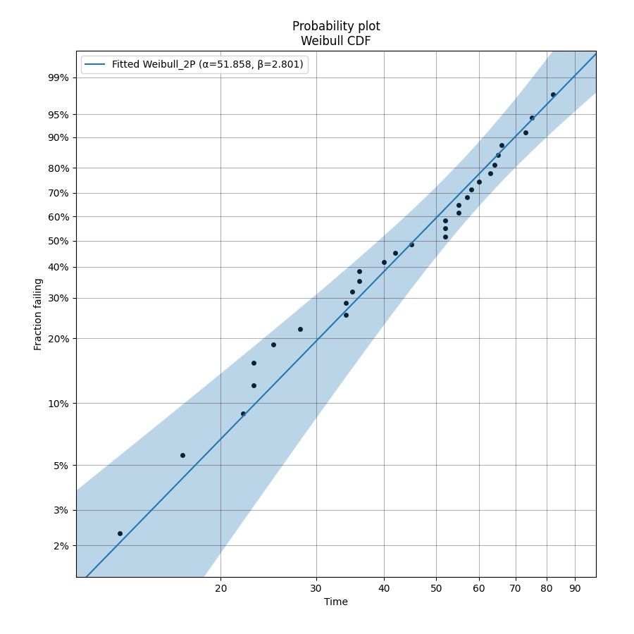
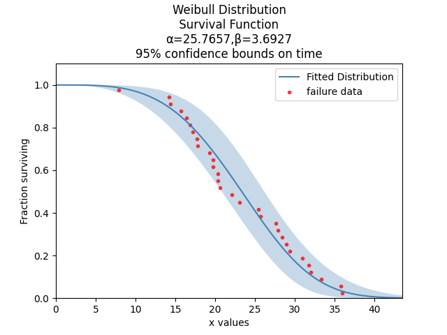
The above probability plot is the typical way to visualise how the CDF (the blue line) models the failure data (the black points). If you would like to view the failure points alongside the PDF, CDF, SF, HF, or CHF without the axis being scaled then you can generate the scatter plot using the function plot_points which is available within reliability.Probability_plotting. In the example below we create some data, then fit a Weibull distribution to the data (ensuring we turn off the probability plot). From the fitted distribution object we plot the Survival Function (SF). We then use plot_points to generate a scatter plot of the plotting positions for the survival function.
API Reference
For inputs and outputs of the plot_points function see the API reference.
Example 2
This example shows how to use the plot_points function.
from reliability.Distributions import Weibull_Distribution
from reliability.Fitters import Fit_Weibull_2P
from reliability.Probability_plotting import plot_points
import matplotlib.pyplot as plt

data = Weibull_Distribution(alpha=25,beta=4).random_samples(30)
weibull_fit = Fit_Weibull_2P(failures=data,show_probability_plot=False,print_results=False)
weibull_fit.distribution.SF(label='Fitted Distribution',color='steelblue')
plot_points(failures=data,func='SF',label='failure data',color='red',alpha=0.7)
plt.legend()
plt.show()
Example 3
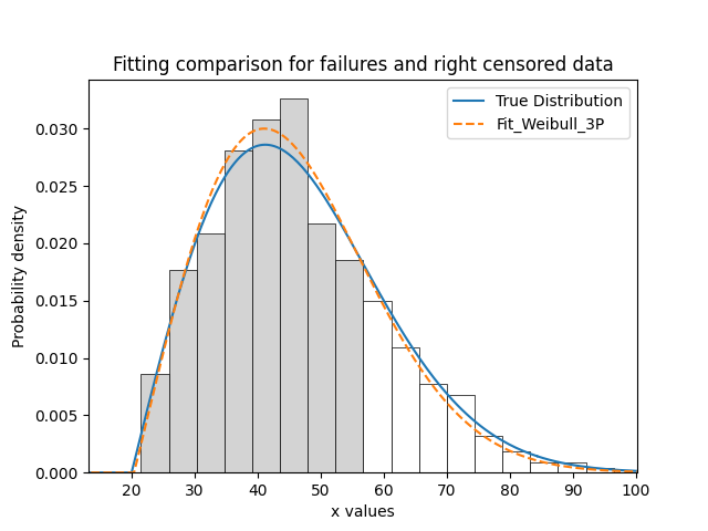
It is beneficial to see the effectiveness of the fitted distribution in comparison to the original distribution. In this example, we are creating 500 samples from a Weibull distribution and then we will right censor all of the data above our chosen threshold. Then we are fitting a Weibull_3P distribution to the data. Note that we need to specify “show_probability_plot=False, print_results=False” in the Fit_Weibull_3P to prevent the normal outputs of the fitting function from being displayed.
from reliability.Distributions import Weibull_Distribution
from reliability.Fitters import Fit_Weibull_3P
from reliability.Other_functions import make_right_censored_data, histogram
import matplotlib.pyplot as plt

a = 30
b = 2
g = 20
threshold=55
dist = Weibull_Distribution(alpha=a, beta=b, gamma=g) # generate a weibull distribution
raw_data = dist.random_samples(500, seed=2)  # create some data from the distribution
data = make_right_censored_data(raw_data,threshold=threshold) #right censor some of the data
print('There are', len(data.right_censored), 'right censored items.')
wbf = Fit_Weibull_3P(failures=data.failures, right_censored=data.right_censored, show_probability_plot=False, print_results=False)  # fit the Weibull_3P distribution
print('Fit_Weibull_3P parameters:\nAlpha:', wbf.alpha, '\nBeta:', wbf.beta, '\nGamma', wbf.gamma)
histogram(raw_data,white_above=threshold) # generates the histogram using optimal bin width and shades the censored part as white
dist.PDF(label='True Distribution')  # plots the true distribution's PDF
wbf.distribution.PDF(label='Fit_Weibull_3P', linestyle='--')  # plots to PDF of the fitted Weibull_3P
plt.title('Fitting comparison for failures and right censored data')
plt.legend()
plt.show()

'''
There are 118 right censored items.
Fit_Weibull_3P parameters:
Alpha: 28.874745169627886
Beta: 2.0294944619390654
Gamma 20.383959629725744
'''
Example 4
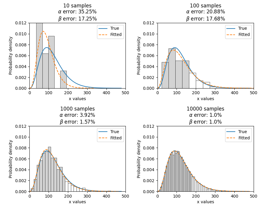
As another example, we will fit a Gamma_2P distribution to some partially right censored data. To provide a comparison of the fitting accuracy as the number of samples increases, we will do the same experiment with varying sample sizes. The results highlight that the accuracy of the fit is proportional to the amount of samples, so you should always try to obtain more data if possible.
from reliability.Distributions import Gamma_Distribution
from reliability.Fitters import Fit_Gamma_2P
from reliability.Other_functions import make_right_censored_data, histogram
import matplotlib.pyplot as plt

a = 30
b = 4
threshold = 180  # this is used when right censoring the data
trials = [10, 100, 1000, 10000]
subplot_id = 221
plt.figure(figsize=(9, 7))
for sample_size in trials:
    dist = Gamma_Distribution(alpha=a, beta=b)
    raw_data = dist.random_samples(sample_size, seed=2)  # create some data. Seeded for repeatability
    data = make_right_censored_data(raw_data, threshold=threshold)  # right censor the data
    gf = Fit_Gamma_2P(failures=data.failures, right_censored=data.right_censored, show_probability_plot=False, print_results=False)  # fit the Gamma_2P distribution
    print('\nFit_Gamma_2P parameters using', sample_size, 'samples:', '\nAlpha:', gf.alpha, '\nBeta:', gf.beta)  # print the results
    plt.subplot(subplot_id)
    histogram(raw_data,white_above=threshold) # plots the histogram using optimal bin width and shades the right censored part white
    dist.PDF(label='True')  # plots the true distribution
    gf.distribution.PDF(label='Fitted', linestyle='--')  # plots the fitted Gamma_2P distribution
    plt.title(str(str(sample_size) + ' samples\n' + r'$\alpha$ error: ' + str(round(abs(gf.alpha - a) / a * 100, 2)) + '%\n' + r'$\beta$ error: ' + str(round(abs(gf.beta - b) / b * 100, 2)) + '%'))
    plt.ylim([0, 0.012])
    plt.xlim([0, 500])
    plt.legend()
    subplot_id += 1
plt.subplots_adjust(left=0.11, bottom=0.08, right=0.95, top=0.89, wspace=0.33, hspace=0.58)
plt.show()

'''
Fit_Gamma_2P parameters using 10 samples:
Alpha: 19.42603577754394
Beta: 4.6901283424759255

Fit_Gamma_2P parameters using 100 samples:
Alpha: 36.26411284656554
Beta: 3.2929448936077534

Fit_Gamma_2P parameters using 1000 samples:
Alpha: 28.825423280158407
Beta: 4.062909060146121

Fit_Gamma_2P parameters using 10000 samples:
Alpha: 30.301232862075587
Beta: 3.96009153189253
'''
Example 5
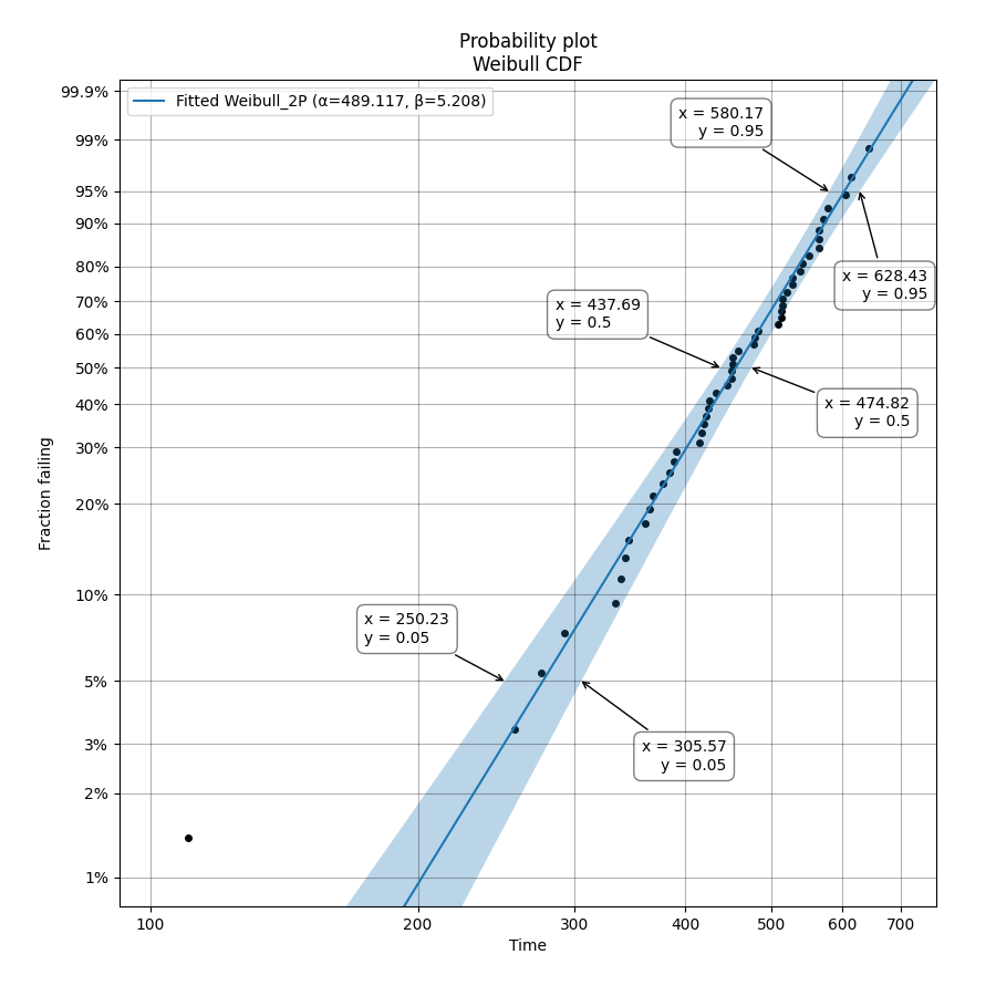
To obtain details of the quantiles (y-values from the CDF) which include the lower estimate, point estimate, and upper estimate, we can use the quantiles input for each Fitter. In this example, we will create some data and fit a Weibull_2P distribution. When quantiles is specified the results printed includes both the table of results and the table of quantiles. Setting quantiles as True will use a default list of quantiles (as shown in the first output). Alternatively we can specify the exact quantiles to use (as shown in the second output). The use of the crosshairs function is also shown which was used to annotate the plot manually. Note that the quantiles provided are the quantiles of the confidence bounds on time. You can extract the confidence bounds on on reliability using the fitted distribution object as shown here.
from reliability.Distributions import Weibull_Distribution
from reliability.Fitters import Fit_Weibull_2P
from reliability.Other_functions import crosshairs
import matplotlib.pyplot as plt

dist = Weibull_Distribution(alpha=500, beta=6)
data = dist.random_samples(50, seed=1)  # generate some data
# this will produce the large table of quantiles below the first table of results
Fit_Weibull_2P(failures=data, quantiles=True, CI=0.8, show_probability_plot=False)
print('----------------------------------------------------------')
# repeat the process but using specified quantiles.
output = Fit_Weibull_2P(failures=data, quantiles=[0.05, 0.5, 0.95], CI=0.8)
# these points have been manually annotated on the plot using crosshairs
crosshairs()
plt.show()

# the values from the quantiles dataframe can be extracted using pandas:
lower_estimates = output.quantiles['Lower Estimate'].values
print('Lower estimates:', lower_estimates)

#alternatively, the bounds can be extracted from the distribution object
lower,point,upper = output.distribution.CDF(CI_y=[0.05, 0.5, 0.95], CI=0.8)
print('Upper estimates:', upper)

'''
Results from Fit_Weibull_2P (80% CI):
Analysis method: Maximum Likelihood Estimation (MLE)
Optimizer: TNC
Failures / Right censored: 50/0 (0% right censored)

Parameter  Point Estimate  Standard Error  Lower CI  Upper CI
    Alpha         489.117         13.9217   471.597   507.288
     Beta         5.20798        0.589269     4.505   6.02066

Goodness of fit    Value
 Log-likelihood -301.658
           AICc  607.571
            BIC   611.14
             AD  0.48267

Table of quantiles (80% CI bounds on time):
 Quantile  Lower Estimate  Point Estimate  Upper Estimate
     0.01         175.215         202.212         233.368
     0.05         250.235         276.521         305.569
      0.1         292.686         317.508         344.435
      0.2         344.277         366.719         390.623
     0.25         363.578          385.05          407.79
      0.5          437.69         455.879         474.824
     0.75          502.94         520.776         539.245
      0.8         517.547         535.917         554.938
      0.9         553.267         574.068         595.651
     0.95         580.174          603.82          628.43
     0.99         625.682          655.79         687.347

----------------------------------------------------------
Results from Fit_Weibull_2P (80% CI):
Analysis method: Maximum Likelihood Estimation (MLE)
Optimizer: TNC
Failures / Right censored: 50/0 (0% right censored)

Parameter  Point Estimate  Standard Error  Lower CI  Upper CI
    Alpha         489.117         13.9217   471.597   507.288
     Beta         5.20798        0.589269     4.505   6.02066

Goodness of fit    Value
 Log-likelihood -301.658
           AICc  607.571
            BIC   611.14
             AD  0.48267

Table of quantiles (80% CI bounds on time):
 Quantile  Lower Estimate  Point Estimate  Upper Estimate
     0.05         250.235         276.521         305.569
      0.5          437.69         455.879         474.824
     0.95         580.174          603.82          628.43

Lower estimates: [250.23461473 437.69015375 580.17421254]
Upper estimates: [305.56872227 474.82362169 628.43042835]
'''
Using Fit_Weibull_2P_grouped for large data sets
The function Fit_Weibull_2P_grouped is effectively the same as Fit_Weibull_2P, except for a few small differences that make it more efficient at handling grouped data sets. Grouped data sets are typically found in very large data that may be heavily censored. The function includes a choice between two optimizers and a choice between two initial guess methods for the initial guess that is given to the optimizer. These help in cases where the data is very heavily censored (>99.9%). The defaults for these options are usually the best but you may want to try different options to see which one gives you the lowest log-likelihood.
API Reference
For inputs and outputs see the API reference.
Example 6
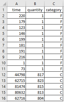
The following example shows how we can use Fit_Weibull_2P_grouped to fit a Weibull_2P distribution to grouped data from a spreadsheet (shown below) on the Windows desktop. If you would like to access this data, it is available in reliability.Datasets.electronics and includes both the failures and right_censored format as well as the dataframe format. An example of this is provided in the code below (option 2).
from reliability.Fitters import Fit_Weibull_2P_grouped
import pandas as pd

# option 1 for importing this dataset (from an excel file on your desktop)
filename = 'C:\\Users\\Current User\\Desktop\\data.xlsx'
df = pd.read_excel(io=filename)

## option 2 for importing this dataset (from the dataset in reliability)
# from reliability.Datasets import electronics
# df = electronics().dataframe

print(df.head(15),'\n')
Fit_Weibull_2P_grouped(dataframe=df, show_probability_plot=False)

'''
     time  quantity category
0     220         1        F
1     179         1        F
2     123         1        F
3     146         1        F
4     199         1        F
5     181         1        F
6     191         1        F
7     216         1        F
8       1         1        F
9      73         1        F
10  44798       817        C
11  62715       823        C
12  81474       815        C
13  80632       813        C
14  62716       804        C

Results from Fit_Weibull_2P_grouped (95% CI):
Analysis method: Maximum Likelihood Estimation (MLE)
Optimizer: TNC
Failures / Right censored: 10/4072 (99.75502% right censored)

Parameter  Point Estimate  Standard Error    Lower CI    Upper CI
    Alpha     6.19454e+21      7.7592e+22 1.34889e+11 2.84473e+32
     Beta        0.153742       0.0485886   0.0827523    0.285632

Goodness of fit    Value
 Log-likelihood -144.617
           AICc  293.236
            BIC  305.862
             AD  264.999
'''