Mean cumulative function
The Mean Cumulative Function (MCF) is a cumulative history function that shows the cumulative number of recurrences of an event, such as repairs over time. In the context of repairs over time, the value of the MCF can be thought of as the average number of repairs that each system will have undergone after a certain time. It is only applicable to repairable systems and assumes that each event (repair) is identical. For the non-parametric MCF it does not assume that each system’s MCF is identical, but this assumption is made for the parametric MCF.
The shape of the MCF is a key indicator that shows whether the systems are improving, worsening, or staying the same over time. If the MCF is concave down (appearing to level out) then the system is improving. A straight line (constant increase) indicates it is staying the same. Concave up (getting steeper) shows the system is worsening as repairs are required more frequently as time progresses.
Obtaining the MCF from failure times is an inherently non-parametric process (similar to Kaplan-Meier), but once the values are obtained, a model can be fitted to obtain the parametric estimate of the MCF. Each of these two approaches is described below as they are performed by seperate functions within reliability.Repairable_systems.
Note that in some textbooks and academic papers the Mean Cumulative Function is also referred to as the Cumulative Intensity Function (CIF). These are two names for the same thing. If the shape of your MCF is more of an S than a single smooth curve, you may have a change in operating condition or in the repair effectiveness factor. This can be dealt with by splitting the MCF into segments, however, such models are more complex and are generally only found in academic literature.
Non-parametric MCF
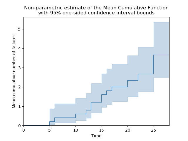
The non-parametric estimate of the MCF provides both the estimate of the MCF and the confidence bounds at a particular time. The procedure to obtain the non-parametric MCF is outlined here. The confidence bounds are the one-sided bounds as this was chosen to align with the method used by Reliasoft.
API Reference
For inputs and outputs see the API reference.
Example 1
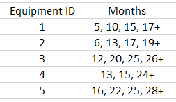
The following example is taken from an example provided by Reliasoft. The failure times and retirement times (retirement time is indicated by +) of 5 systems are:
from reliability.Repairable_systems import MCF_nonparametric
import matplotlib.pyplot as plt
times = [[5, 10, 15, 17], [6, 13, 17, 19], [12, 20, 25, 26], [13, 15, 24], [16, 22, 25, 28]]
MCF_nonparametric(data=times)
plt.show()

'''
Mean Cumulative Function results (95% CI):
state  time MCF_lower     MCF MCF_upper variance
    F     5 0.0459299     0.2  0.870893    0.032
    F     6   0.14134     0.4   1.13202    0.064
    F    10  0.256603     0.6   1.40294    0.096
    F    12  0.383374     0.8   1.66939    0.128
    F    13  0.517916       1   1.93081     0.16
    F    13  0.658169     1.2   2.18789    0.192
    F    15  0.802848     1.4   2.44131    0.224
    F    15  0.951092     1.6   2.69164    0.256
    F    16   1.10229     1.8   2.93935    0.288
    F    17   1.25598       2   3.18478     0.32
    C    17
    C    19
    F    20   1.49896 2.33333   3.63215 0.394074
    F    22   1.74856 2.66667   4.06684 0.468148
    C    24
    F    25   2.12259 3.16667   4.72431 0.593148
    F    25    2.5071 3.66667   5.36255 0.718148
    C    26
    C    28


'''
Parametric MCF
The estimates of the parametric MCF are obtained using MCF_nonparametric as this is the procedure required to obtain the points for the plot. We use these points to fit a Non-Homogeneous Poisson Process (NHPP) parametric model of the form:
\(MCF(t) = (\frac{t}{\alpha})^{\beta}\)
You may notice that this looks identical to the Weibull CHF, but despite this similarity, they are entirely different functions and the alpha and beta parameters from the MCF cannot be applied to a Weibull distribution for fitting the repair times or repair interarrival times.
The purpose of fitting a parametric model is to obtain the shape parameter (β) which indicates the long term health of the system/s. If the MCF is concave down (β<1) then the system is improving. A straight line (β=1) indicates it is staying the same. Concave up (β>1) shows the system is worsening as repairs are required more frequently as time progresses.
Many methods exist for fitting the model to the data. Within reliability, scipy.optimize.curve_fit is used which returns the covariance matrix and allows for the confidence intervals to be calculated using the appropriate formulas.
API Reference
For inputs and outputs see the API reference.
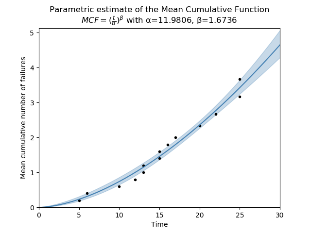
Example 2
The following example uses the same data as the MCF_nonparametric example provided above. From the output we can clearly see that the system is degrading over time as repairs are needed more frequently.
from reliability.Repairable_systems import MCF_parametric
import matplotlib.pyplot as plt
times = [[5, 10, 15, 17], [6, 13, 17, 19], [12, 20, 25, 26], [13, 15, 24], [16, 22, 25, 28]]
MCF_parametric(data=times)
plt.show()

'''
Mean Cumulative Function Parametric Model (95% CI):
MCF = (t/α)^β
Parameter  Point Estimate  Standard Error  Lower CI  Upper CI
    Alpha         11.9806        0.401372   11.2192   12.7937
     Beta         1.67362       0.0946537   1.49802   1.86981

Since Beta is greater than 1, the system repair rate is WORSENING over time.
'''
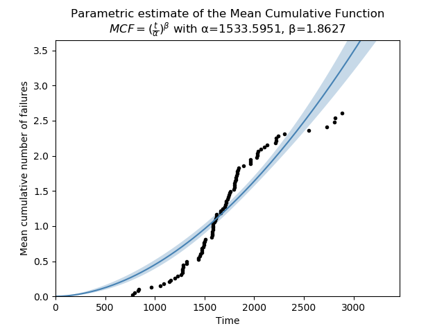
Example 3
The parametric model that is fitted to the MCF is not always an appropriate model. The example below shows data from a collection of systems, some of which are improving and some are worsening. The net effect is an S-shaped MCF. The power model used by MCF_parametric is not able to accurately follow an S-shaped dataset. In this case, the MCF_nonparametric model is more appropriate, though there are some other parametric models (discussed in the first paragraph) which may be useful to model this dataset.
from reliability.Repairable_systems import MCF_parametric
from reliability.Datasets import MCF_2
import matplotlib.pyplot as plt

times = MCF_2().times
MCF_parametric(data=times, print_results=False)
plt.show()