Fitting a single stress model to ALT data
Before reading this section it is recommended that readers are familiar with the concepts of fitting probability distributions, probability plotting, and have an understanding of what accelerated life testing (ALT) involves.
The module reliability.ALT_fitters contains 24 ALT models; 12 of these models are for single stress and 12 are for dual stress. This section details the single stress models, though the process for fitting dual-stress models is similar. The decision to use a single stress or dual stress model depends entirely on your data. If your data only has one stress that is being changed then you will use a single stress model.
The following single stress models are available within ALT_fitters:
Fit_Weibull_Exponential
Fit_Weibull_Eyring
Fit_Weibull_Power
Fit_Lognormal_Exponential
Fit_Lognormal_Eyring
Fit_Lognormal_Power
Fit_Normal_Exponential
Fit_Normal_Eyring
Fit_Normal_Power
Fit_Exponential_Exponential
Fit_Exponential_Eyring
Fit_Exponential_Power
API Reference
For inputs and outputs see the API reference.
Example 1
In the following example, we will fit the Weibull-Power model to an ALT dataset obtained from a fatigue test. This dataset can be found in reliability.Datasets. We want to know the mean life at the use level stress of 60 so the parameter use_level_stress is specified. All other values are left as defaults and the results and plot are shown.
from reliability.ALT_fitters import Fit_Weibull_Power
from reliability.Datasets import ALT_load2
import matplotlib.pyplot as plt

Fit_Weibull_Power(failures=ALT_load2().failures, failure_stress=ALT_load2().failure_stresses, right_censored=ALT_load2().right_censored, right_censored_stress=ALT_load2().right_censored_stresses, use_level_stress=60)
plt.show()

'''
Results from Fit_Weibull_Power (95% CI):
Analysis method: Maximum Likelihood Estimation (MLE)
Optimizer: TNC
Failures / Right censored: 13/5 (27.77778% right censored)

Parameter  Point Estimate  Standard Error  Lower CI   Upper CI
        a          393440          508989   31166.6 4.9667e+06
        n        -1.41476        0.242371   -1.8898  -0.939725
     beta         3.01934        0.716268   1.89664    4.80662

 stress  original alpha  original beta  new alpha  common beta beta change  acceleration factor
    300         116.174        3.01009    123.123      3.01934      +0.31%              9.74714
    200         240.182        3.57635    218.507      3.01934     -15.57%              5.49224
    100          557.42         2.6792    582.575      3.01934      +12.7%              2.05998

 Goodness of fit    Value
 Log-likelihood -76.8542
           AICc  161.423
            BIC  162.379

At the use level stress of 60, the mean life is 1071.96438
'''
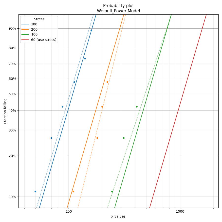
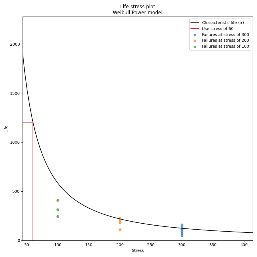
In the results above we see 3 tables of results; the fitted parameters (along with their confidence bounds) dataframe, the change of parameters dataframe, and the goodness of fit dataframe. For the change of parameters dataframe the “original alpha” and “original beta” are the fitted values for the Weibull_2P distribution that is fitted to the data at each stress (shown on the probability plot by the dashed lines). The “new alpha” and “new beta” are from the Weibull_Power model. The beta change is extremely important as it allows us to identify whether the fitted ALT model is appropriate at each stress level. A beta change of over 50% will trigger a warning to be printed informing the user that the failure mode may be changing across different stresses, or that the model is inappropriate for the data. The acceleration factor column will only be returned if the use level stress is provided since acceleration factor is a comparison of the life at the higher stress vs the use stress.
Example 2
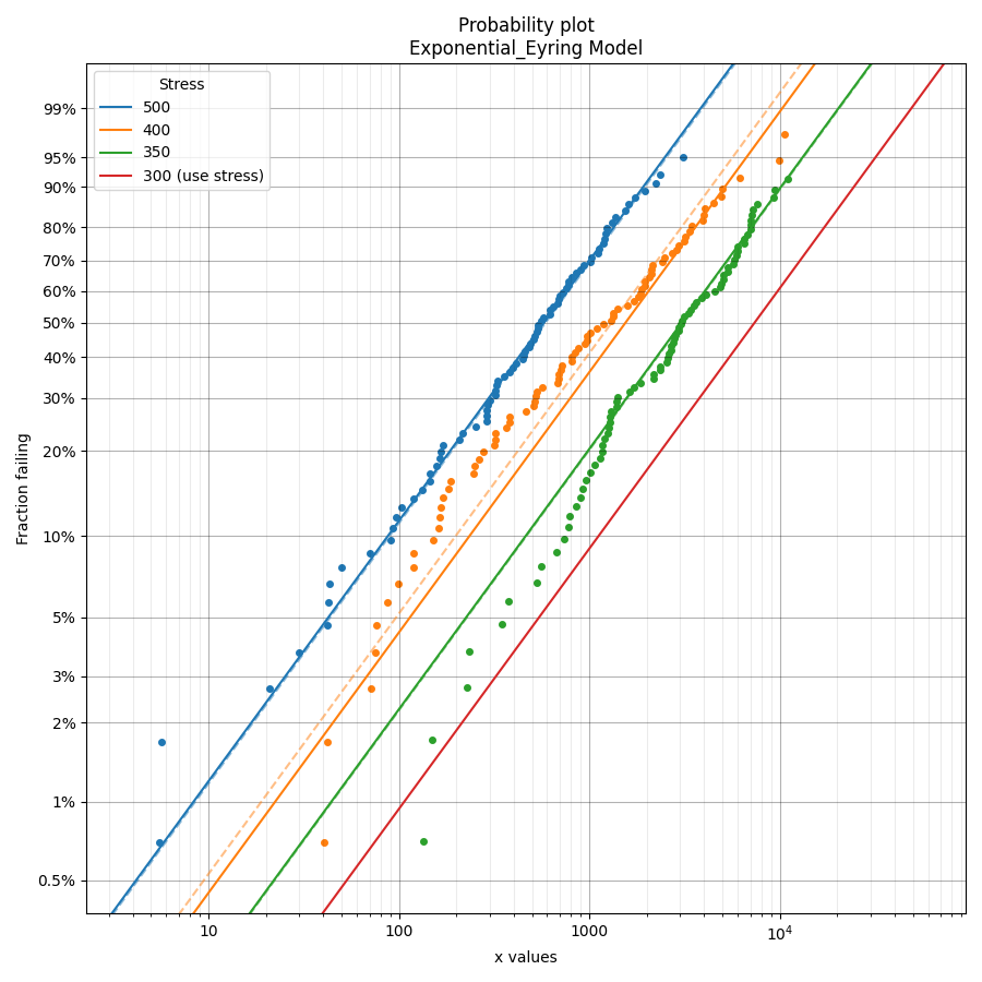
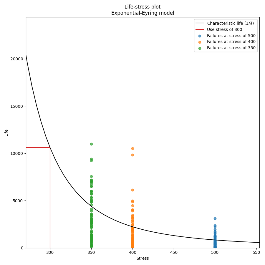
In this second example we will fit the Exponential-Eyring model. Instead of using an existing dataset we will create our own data using the function make_ALT_data. Since the Exponential_1P distribution has only 1 parameter (Lambda), the function fits a Weibull_2P distribution and then compares the change of parameters of the Weibull alpha and beta with the Exponential 1/Lambda (obtained from the life-stress model) and the shape parameter of 1 (since a Weibull distrbution with beta=1 is equivalent to the Exponential distribution). This provides similar functionality for examining the change of parameters as we find with the models for all the other distributions (Weibull, Lognormal, and Normal).
The results show that the fitted parameters agree well with the parameters we used to generate the data, as does the mean life at the use stress. This accuracy improves with more data.
from reliability.Other_functions import make_ALT_data
from reliability.ALT_fitters import Fit_Exponential_Eyring
import matplotlib.pyplot as plt

use_level_stress = 300
ALT_data = make_ALT_data(distribution='Exponential',life_stress_model='Eyring',a=1500,c=-10,stress_1=[500,400,350],number_of_samples=100,fraction_censored=0.2,seed=1,use_level_stress=use_level_stress)
Fit_Exponential_Eyring(failures=ALT_data.failures, failure_stress=ALT_data.failure_stresses, right_censored=ALT_data.right_censored, right_censored_stress=ALT_data.right_censored_stresses, use_level_stress=use_level_stress)
print('The mean life at use stress of the true model is:',ALT_data.mean_life_at_use_stress)
plt.show()

'''
Results from Fit_Exponential_Eyring (95% CI):
Analysis method: Maximum Likelihood Estimation (MLE)
Optimizer: TNC
Failures / Right censored: 240/60 (20% right censored)

Parameter  Point Estimate  Standard Error  Lower CI  Upper CI
        a         1428.47         178.875   1077.88   1779.06
        c        -10.2599        0.443394  -11.1289  -9.39085

 stress  weibull alpha  weibull beta  new 1/Lambda  common shape shape change  acceleration factor
    500        1034.22      0.981495       994.473             1       +1.89%              11.1948
    400        2149.92      0.877218       2539.17             1       +14.0%              4.38449
    350        5251.88       1.07081       4833.32             1       -6.61%              2.30337

 Goodness of fit    Value
 Log-likelihood -2098.01
           AICc  4200.06
            BIC  4207.42

At the use level stress of 300, the mean life is 11132.94095

The mean life at use stress of the true model is: 10896.724574907037
'''
Example 3
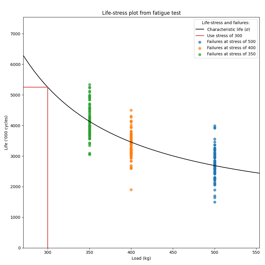
In this third example, we will look at how to customise the labels on the plots. Two of the outputs returned are the axes handles for the probability plot and the life-stress plot. These handles can be used to set certain values such as xlabel, ylabel, title, legend title, etc. For simplicity in this example the printing of results and the probability plot are turned off so the only output is the life-stress plot.
from reliability.Other_functions import make_ALT_data
from reliability.ALT_fitters import Fit_Normal_Exponential
import matplotlib.pyplot as plt

ALT_data = make_ALT_data(distribution='Normal',life_stress_model='Exponential',a=500,b=1000,sigma=500,stress_1=[500,400,350],number_of_samples=100,fraction_censored=0.2,seed=1)
# the results and probability plot have been turned off so we just get the life-stress plot
model = Fit_Normal_Exponential(failures=ALT_data.failures, failure_stress=ALT_data.failure_stresses, right_censored=ALT_data.right_censored, right_censored_stress=ALT_data.right_censored_stresses, use_level_stress=300, print_results=False, show_probability_plot=False)
# customize the life-stress plot labels
model.life_stress_plot.set_xlabel('Load (kg)')
model.life_stress_plot.set_ylabel("Life ('000 cycles)")
model.life_stress_plot.set_title('Life-stress plot from fatigue test')
model.life_stress_plot.legend(title='Life-stress and failures:')
plt.show()
References:
Probabilistic Physics of Failure Approach to Reliability (2017), by M. Modarres, M. Amiri, and C. Jackson. pp. 136-168
Accelerated Life Testing Data Analysis Reference - ReliaWiki, Reliawiki.com, 2019. [Online].