Kaplan-Meier
API Reference
For inputs and outputs see the API reference.
The Kaplan-Meier estimator provides a method by which to estimate the survival function (reliability function) of a population without assuming that the data comes from a particular distribution. Due to the lack of parameters required in this model, it is a non-parametric method of obtaining the survival function. With a few simple transformations, the survival function (SF) can be used to obtain the cumulative hazard function (CHF) and the cumulative distribution function (CDF). It is not possible to obtain a useful version of the probability density function (PDF) or hazard function (HF) as this would require the differentiation of the CDF and CHF respectively, which results in a very spikey plot due to the non-continuous nature of these plots.
The Kaplan-Meier estimator is very similar in result (but quite different in method) to the Nelson-Aalen estimator and Rank Adjustment estimator. While none of the three has been proven to be more accurate than the others, the Kaplan-Meier estimator is generally more popular as a non-parametric means of estimating the SF. Confidence intervals are provided using the Greenwood method with Normal approximation.
The Kaplan-Meier estimator can be used with both complete and right censored data. This function can be accessed from reliability.Nonparametric.KaplanMeier.
Example 1
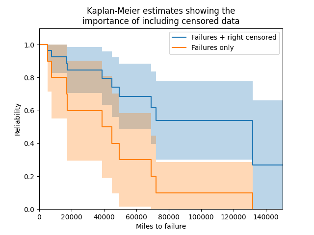
In this first example, we will provide Kaplan-Meier with a list of failure times and right censored times. By leaving everything else unspecified, the plot will be shown with the confidence intervals shaded. We will layer this first Kaplan-Meier plot with a second one using just the failure data. As can be seen in the example below, the importance of including censored data is paramount to obtain an accurate estimate of the reliability, because without it the population’s survivors are not included so the reliability will appear much lower than it truly is.
from reliability.Nonparametric import KaplanMeier
import matplotlib.pyplot as plt
f = [5248, 7454, 16890, 17200, 38700, 45000, 49390, 69040, 72280, 131900]
rc = [3961, 4007, 4734, 6054, 7298, 10190, 23060, 27160, 28690, 37100, 40060, 45670, 53000, 67000, 69630, 77350, 78470, 91680, 105700, 106300, 150400]
KaplanMeier(failures=f, right_censored=rc, label='Failures + right censored')
KaplanMeier(failures=f, label='Failures only')
plt.title('Kaplan-Meier estimates showing the\nimportance of including censored data')
plt.xlabel('Miles to failure')
plt.legend()
plt.show()

'''
Results from KaplanMeier (95% CI):
 Failure times  Censoring code (censored=0)  Items remaining  Kaplan-Meier Estimate  Lower CI bound  Upper CI bound
          3961                            0               31                      1               1               1
          4007                            0               30                      1               1               1
          4734                            0               29                      1               1               1
          5248                            1               28               0.964286        0.895548               1
          6054                            0               27               0.964286        0.895548               1
          7298                            0               26               0.964286        0.895548               1
          7454                            1               25               0.925714        0.826513               1
         10190                            0               24               0.925714        0.826513               1
         16890                            1               23               0.885466         0.76317               1
         17200                            1               22               0.845217        0.705334        0.985101
         23060                            0               21               0.845217        0.705334        0.985101
         27160                            0               20               0.845217        0.705334        0.985101
         28690                            0               19               0.845217        0.705334        0.985101
         37100                            0               18               0.845217        0.705334        0.985101
         38700                            1               17               0.795499        0.633417         0.95758
         40060                            0               16               0.795499        0.633417         0.95758
         45000                            1               15               0.742465        0.560893        0.924037
         45670                            0               14               0.742465        0.560893        0.924037
         49390                            1               13               0.685353         0.48621        0.884496
         53000                            0               12               0.685353         0.48621        0.884496
         67000                            0               11               0.685353         0.48621        0.884496
         69040                            1               10               0.616817        0.396904        0.836731
         69630                            0                9               0.616817        0.396904        0.836731
         72280                            1                8               0.539715        0.300949        0.778481
         77350                            0                7               0.539715        0.300949        0.778481
         78470                            0                6               0.539715        0.300949        0.778481
         91680                            0                5               0.539715        0.300949        0.778481
        105700                            0                4               0.539715        0.300949        0.778481
        106300                            0                3               0.539715        0.300949        0.778481
        131900                            1                2               0.269858               0        0.662446
        150400                            0                1               0.269858               0        0.662446

Results from KaplanMeier (95% CI):
 Failure times  Censoring code (censored=0)  Items remaining  Kaplan-Meier Estimate  Lower CI bound  Upper CI bound
          5248                            1               10                    0.9        0.714061               1
          7454                            1                9                    0.8        0.552082               1
         16890                            1                8                    0.7        0.415974        0.984026
         17200                            1                7                    0.6        0.296364        0.903636
         38700                            1                6                    0.5        0.190102        0.809898
         45000                            1                5                    0.4       0.0963637        0.703636
         49390                            1                4                    0.3       0.0159742        0.584026
         69040                            1                3                    0.2               0        0.447918
         72280                            1                2                    0.1               0        0.285939
        131900                            1                1                      0               0               0
'''
Example 2
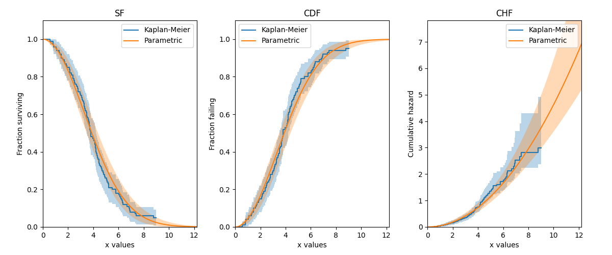
In this second example, we will create some data from a Weibull distribution, and then right censor the data above our chosen threshold. We will then fit a Weibull_2P distribution to the censored data, and also obtain the Kaplan-Meier estimate of this data. Using the results from the Fit_Weibull_2P and the Kaplan-Meier estimate, we will plot the CDF, SF, and CHF, for both the Weibull and Kaplan-Meier results. Note that the default plot from KaplanMeier will only give you the SF, but the results object provides everything you need to reconstruct the SF plot yourself, as well as what we need to plot the CDF and CHF.
from reliability.Distributions import Weibull_Distribution
from reliability.Fitters import Fit_Weibull_2P
from reliability.Nonparametric import KaplanMeier
from reliability.Other_functions import make_right_censored_data
import matplotlib.pyplot as plt

dist = Weibull_Distribution(alpha=5, beta=2)  # create a distribution
raw_data = dist.random_samples(100, seed=2)  # get some data from the distribution. Seeded for repeatability
data = make_right_censored_data(raw_data, threshold=9)
wbf = Fit_Weibull_2P(failures=data.failures, right_censored=data.right_censored, show_probability_plot=False, print_results=False)  # Fit the Weibull_2P

# Create the subplots and in each subplot we will plot the parametric distribution and obtain the Kaplan Meier fit.
# Note that the plot_type is being changed each time
plt.figure(figsize=(12, 5))
plt.subplot(131)
KaplanMeier(failures=data.failures, right_censored=data.right_censored, plot_type='SF', print_results=False, label='Kaplan-Meier')
wbf.distribution.SF(label='Parametric')
plt.legend()
plt.title('SF')
plt.subplot(132)
KaplanMeier(failures=data.failures, right_censored=data.right_censored, plot_type='CDF', print_results=False, label='Kaplan-Meier')
wbf.distribution.CDF(label='Parametric')
plt.legend()
plt.title('CDF')
plt.subplot(133)
KaplanMeier(failures=data.failures, right_censored=data.right_censored, plot_type='CHF', print_results=False, label='Kaplan-Meier')
wbf.distribution.CHF(label='Parametric')
plt.legend()
plt.title('CHF')
plt.subplots_adjust(left=0.07, right=0.95, top=0.92, wspace=0.25)  # format the plot layout
plt.show()