Quickstart for reliability
Installation and upgrading
If you are new to using Python, you will first need to install a Python 3 interpreter and also install an IDE so that you can interact with the code. There are many good IDEs available including Pycharm, Spyder and Jupyter.
Once you have Python installed, to install reliability for the first time, open your command prompt and type:
pip install reliability
To upgrade a previous installation of reliability to the most recent version, open your command prompt and type:
pip install --upgrade reliability
If you would like to be notified by email of when a new release of reliability is uploaded to PyPI, there is a free service to do exactly that called NewReleases.io.
A quick example
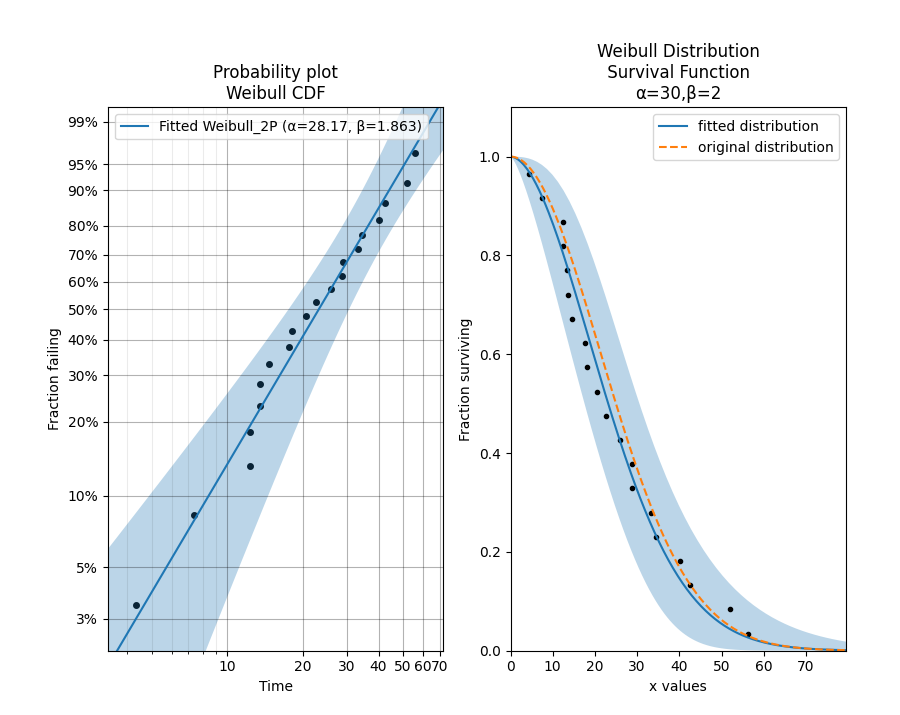
In this example, we will create a Weibull Distribution, and from that distribution we will draw 20 random samples. Using those samples we will Fit a 2-parameter Weibull Distribution. The fitting process generates the probability plot. We can then access the distribution object to plot the survival function.
from reliability.Distributions import Weibull_Distribution
from reliability.Fitters import Fit_Weibull_2P
from reliability.Probability_plotting import plot_points
import matplotlib.pyplot as plt

dist = Weibull_Distribution(alpha=30, beta=2)  # creates the distribution object
data = dist.random_samples(20, seed=42)  # draws 20 samples from the distribution. Seeded for repeatability
plt.subplot(121)
fit = Fit_Weibull_2P(failures=data)  # fits a Weibull distribution to the data and generates the probability plot
plt.subplot(122)
fit.distribution.SF(label='fitted distribution')  # uses the distribution object from Fit_Weibull_2P and plots the survival function
dist.SF(label='original distribution', linestyle='--') # plots the survival function of the original distribution
plot_points(failures=data, func='SF')  # overlays the original data on the survival function
plt.legend()
plt.show()

'''
Results from Fit_Weibull_2P (95% CI):
Analysis method: Maximum Likelihood Estimation (MLE)
Failures / Right censored: 20/0 (0% right censored)

Parameter  Point Estimate  Standard Error  Lower CI  Upper CI
    Alpha         28.1696         3.57032   21.9733   36.1131
     Beta         1.86309         0.32449   1.32428   2.62111

Goodness of fit    Value
 Log-likelihood -79.5482
           AICc  163.802
            BIC  165.088
             AD 0.837278
'''
A key feature of reliability is that probability distributions are created as objects, and these objects have many properties (such as the mean) that are set once the parameters of the distribution are defined. Using the dot operator allows us to access these properties as well as a large number of methods (such as drawing random samples as seen in the example above).
Each distribution may be visualised in five different plots. These are the Probability Density Function (PDF), Cumulative Distribution Function (CDF), Survival Function (SF) [also known as the reliabilty function], Hazard Function (HF), and the Cumulative Hazard Function (CHF). Accessing the plot of any of these is as easy as any of the other methods. Eg. dist.SF() in the above example is what plots the survival function using the distribution object that was returned from the fitter.